The AKF Availability Cube is a model to guide discussions on how to achieve high availability, as well as a tool to evaluate the theoretical "as designed" availability of existing systems. It is the first in a two-part series on designing for high availability. Have a constant problem with low availability? Experiencing re-occurring failures? If so, the AKF Availability Cube and our microservice patterns and anti-patterns may be able to help.
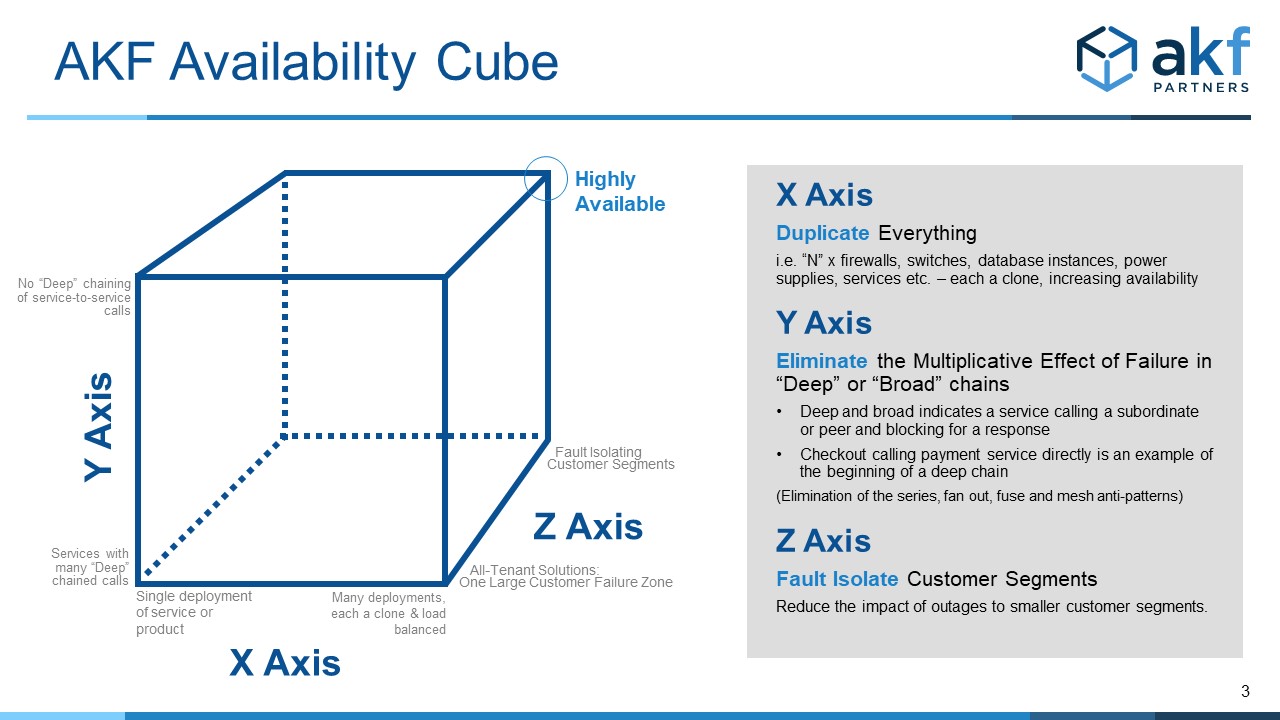
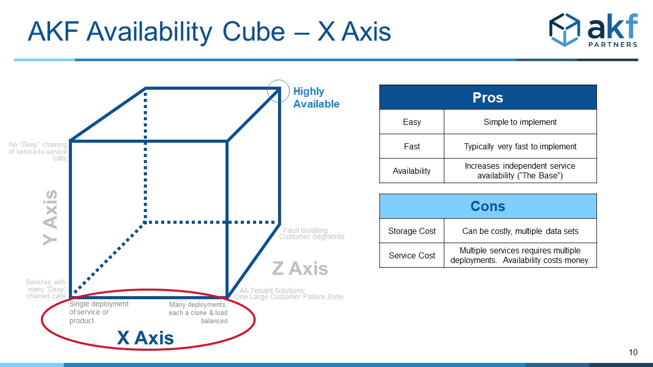
The X Axis of the Availability Cube
Any product/service/solution we develop should have multiple instances (deployments) of the service/product. Just as the X axis of the AKF Scale Cube indicates “cloning/replication” for the ability to scale transactions, so must we clone services (add extra deployments) to increase availability.
Let’s say that we estimate the availability of a single instance of a service (or product) to be 99.99% available. There is a LOT that goes into this estimation – a topic we will discuss in a later post. But for now, let’s assume that we have historical performance and that our application (service/product) has shown a low incidence of failure and low recovery time upon failure. While we prefer not to use time as an availability metric, we will do so here to keep the math familiar to everyone.
We hope to reliably achieve greater than 99.99% available overall, and to do that we add a second node. Here’s where we perform a big leap of faith with math. Time-based availability metrics don’t show the probability of failure – they indicate a simple relationship between the time our solution was available and total possible as in the following:

“Non Available” Time is really a product of both the probability of failure and the mean time to recover from that failure. While strictly mathematically incorrect, we can create a directionally correct availability evaluation by using this product as if it were just the probability. After all, it covers both the probability of a failure AND the average duration of non-availability.
Adding a second node, which should also achieve 99.99% availability then increases our availability because the likelihood that both nodes fail at the same time with our new proxy for probability becomes the probability (1-Availability) that both nodes are down at the same time:
Or
Remember – we’ve cheated by treating the implied probability of failure and MTTR combination as a probability of failure. But it is nevertheless directionally correct. As long as the failure cause is not significantly increased demand, and as long as the availability is derived from perceived operations, we have a decent number with which to work.
This new number now becomes a BASE for an uncertain simple exponential equation.
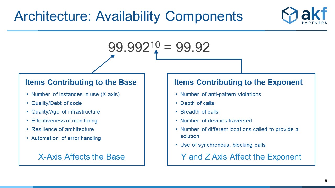
The X axis of our cube shows that increasing the number of instances of a product, monolith, or service increases our overall availability.
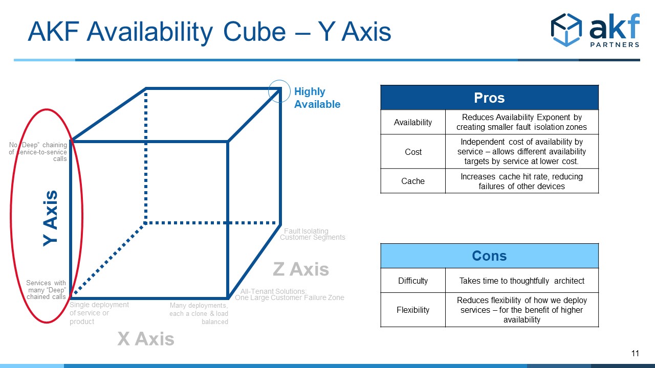
The Y Axis of the Availability Cube
The Y Axis of the Availability Cube is like the Y axis of the AKF Scale Cube in that it addresses fault isolation between services – both in depth and in breadth. More specifically, it is concerned with the number of service and data fan outs, as well as service and data fuses. Mesh interactions also cause a problem.
Unlike the scale cube, “more” of something in the Y axis of the Availability Cube isn’t desirable. As such, the Y axis of the cube moves from a large number to near 0, with high degrees of interservice communication increasing the multiplicative effect of failure https://akfpartners.com/growth..., thereby reducing availability.
The math here is simpler. Anytime we chain (synchronously call in anyway) services, the availability is reduced. If service 1 through service N have a perceived (or theoretical) availability of 99.99%, the availability of the sequence of calls of 1 through N is:
The Y axis then increments the exponent of our availability calculation, as applied to the base determined from the X axis. For any connected services, simply count the number of edges in the service-to-service(s) graph and apply that to the base identified in the X axis calculation above.
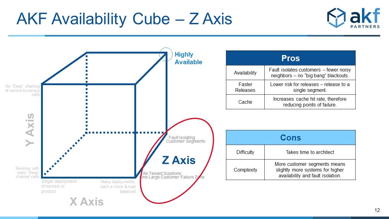
The Z Axis of the Availability Cube
Similar to the Z axis of the Scalability Cube, the Z axis of the Availability Cube defines “blast radius” boundaries (sometimes called Bulkheads in microservices and alternatively called Swimlanes by AKF). Most commonly these boundaries are defined by customer boundaries (groups or segments of customers we serve), geographies of the globe or within a nation, or potentially transaction identifiers within analytics systems. The boundary assumes that no synchronous call that would otherwise increment the exponent as in the Y axis discussion above exists between any swimlane, bulkhead, or blast containment zone.
As such, the Z axis serves to constrain the upper bound for any deployment of the exponent in our availability calculations.
Learn More
Watch our videos on YouTube
Having problems with the availability of your product? Need help designing your next solution for high availability? Give us a call - we can help!