The Relative Risk Equation
Technologists are frequently asked: what are the chances that a given software release is going to work? Do we understand the risk that each component or new feature brings to the entire release?
In this case, measuring risk is assessing the probability that a component will perform poorly or even fail. The higher the probability of failure, the higher the risk. Probabilities are just numbers, so ideally, we should be able to calculate the risk (probability of failure) of the entire release by aggregating the individual risk of each component. In reality this calculation works quite well.
Putting a number to risk is a very useful tool and this article will provide a simple and easy way to calculate risk and produce a numeric result which can be used to compare risk across a spectrum of technology changes.
When we assess a system, one of the key characteristics we want to benchmark is the probability that a system will fail. In particular, if we want to understand whether or not a system can support an availability goal of 99.95% we have to do some analysis to see if the probability that a failure occurs is lower than 0.05%. How do we calculate this?
First let’s introduce some vocabulary.
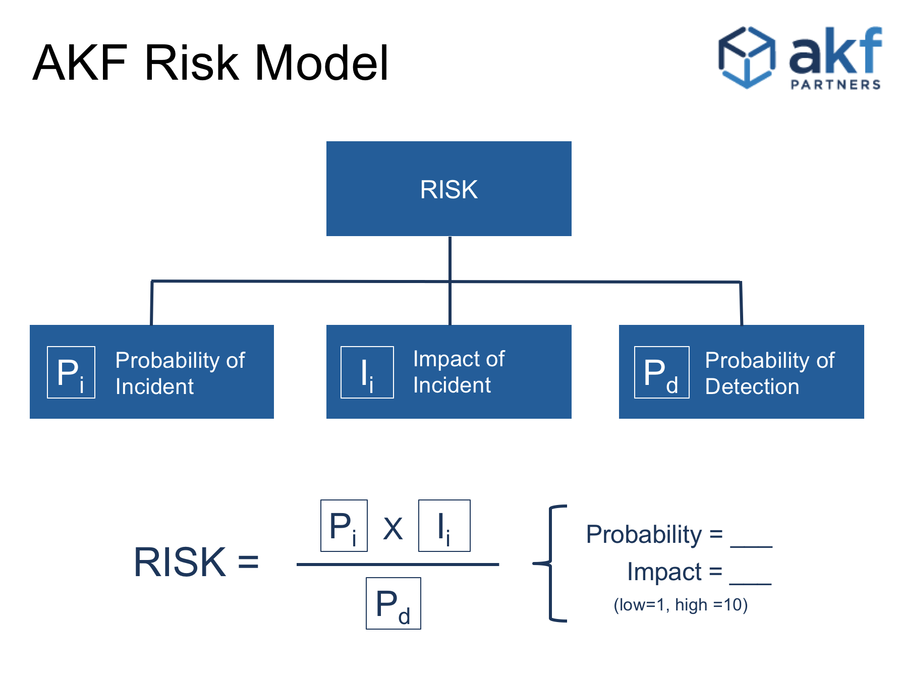
DEFINITION: Pi is the probability that a given system will experience an incident, i.
For the purposes of this article we are measuring relative and not absolute values. A system where Pi=1 means the system is very unlikely to experience failure. On other hand, Pi values approaching 10 indicate a system with a 100% probability of failure.
DEFINITION: Ii is the impact (or blast radius) a system failure will have.
Ii=1 indicated no impact where Ii=10 indicates a complete failure of an entire system.
DEFINITION: Pd is the probability that an incident will be detected.
Pd=1 means an incident will be completely undetected and Pd=10 indicates that a failure will be completely detected 100% of the time.
Measuring across a scale from 1 to 10 is often too granular; we can reduce scale to tee-shirt sizes and replace 1, 2, …, 10 with Small (3), Medium (5), Large (7). Any series of values will work so long as we are consistent in our approach.
Relative Risk is now only a question of math:
Ri = (Pi x Ii ) / Pd
With values of 1, 2, ..., 10, the minimum Relative Risk value is 0.1 (effectively 0 relative risk) and the maximum value is 100. With tee-shirt sizes, the minimum Relative Risk value is 6/7 and the maximum value is 16.333. Basic statistics can help us to standardize values from 1 to 10:
std(Ri) = (Ri - Min(Ri)) / (Max(Ri) - Min(Ri)) x 10
where Max(Ri) = 16 1/3 and Min(Ri) = 1 2/7 (in the case of tee-shirt sizing)
For example:
Example 1: Adding a new data file to a relational database
- Pi = 3 (low.). It’s unlikely that adding a data file will cause a system failure, unless we’re already out of space.
- Ii = 5 (medium.). A failure to add a datafile indicates a larger storage issue may exist which would be very impactful for this database instance. However as there is a backup (for this example), the risk is lowered.
- Pd = 7 (high). It is virtually certain that any failure would be noticed immediately.</li>
- Therefore Ri = (3 X 5) / 7 = 2.1. Standardizing this to our 1 to 10 scale produces a value of 0.51. That is a very low number, so adding datafiles is relatively low risk procedure.
Example 2: Database backups have been stored on tapes that have been demagnetized during transportation to offsite storage.
- Pi = 5 (medium.). While restoring a backup is a relatively safe event, on a production system it is likely happening during a time of maximum stress.
- Ii = 7 (high.). When we attempt to restore the backup tape, it will fail.
- Pd= 3 (low.) The demagnetization of the tapes was a silent and undetected failure.
- Therefore Ri = (5 X 7) / 3 or 11.7. We arrive at a value of 7 on the standard scale, which is quite high, so we should consider randomly testing tapes from off-site storage.
This formula has utility across a vast spectrum of technology:
- Calculate a relative risk value for each feature in a software release, then take the total value of all features in order to compare risk of a release against other releases and consider more detailed testing for higher relative risk values.
- During security risk analysis, calculate a relative risk value for each threat vector and sort the resulting values. The result is a prioritized list of steps required to improve security based on the probabilistic likelihood that a threat vector will cause real damage.
- During feature planning and prioritization exercises, this formula can be altered to calculate feature risk. For example, Pi can mean confidence in estimate, Ii can be converted to impact of feature (e.g. higher revenue = higher impact) and Pd is perceived risk of the feature. Putting all features through this calculation then sorting from high values to low values yields a list of features ranked by value and risk.
The purpose of this formula and similar methods is not to produce a mathematically absolute estimate of risk. The real value here is to remove guessing and emotion from the process of evaluating risk and providing a framework to compare risk across a variety of changes.
Click here to see how AKF Partners can help you manage risk and other technology issues.